Blob Physics – Part 1

Further to the questions we got on our CrazyBites #7, it was clear our followers are interested in more info about blob physics.

Here’s part 1 of the guest post by Laze Ristoski, our Technical Lead:

I’ve had a fun challenge lately. I’ve been doing some experimental work regarding an upcoming game at CrazyLabs that involves rendering and manipulation of 2D bubbles.

My immediate thought was to represent bubbles as hard particles described by their positions and radii, and render them as a Voronoi diagram. This turned out to be unsatisfactory because the hard particles would never provide the fluidity of motion that the game designers had envisioned. The bubbles had to be deformable, and the simple position and radius representation would simply not work.

The next obvious representation, that would help us capture the bubble’s shape at a specific instant of time, would be to hold multiple particles around the bubble’s circumference, and so I looked into soft body physics and blob simulation.

For the purposes of this text, a blob is a jelly-like object that tends to assume a circular shape. This will be the first part in a series where I describe how blob simulation works.

Physics simulation

The high-level physics simulation algorithm is very simple. Here it is in its entirety:

for each particle:

loop numIterations times:

for each particle:

We assume that all of the particles have the same mass and we will not hold this information explicitly as we are only interested in how these masses relate to one another. At first, given the position and velocity of a particle, and a time step, we predict the particle’s future position like this: nextPosition = position + velocity * timeStep. This should be fairly intuitive, but it’s worth emphasizing that the velocity is assumed to be constant during the whole time step. This assumption is false when the particle is affected by forces and constraints. Intuitively, taking smaller time steps yields lower error. A time step of ~33ms (30 FPS) works reasonably well in practice. Note that we do not immediately overwrite the position variable, as we will make use of it in the final step of the algorithm. Afterwards, we simulate friction by keeping a fraction of the particle’s velocity. The value of the damping parameter is tweakable in the range of 0.0 − 1.0, with higher values making for more slippery blobs.

Then comes the tricky part of the algorithm where we apply various constraints to the particles. This is what makes the individual particles work as a cohesive whole. We resolve constraints by moving the particles around (modifying their nextPosition variable). For the purpose of simulating blobs, a few types of constraints come into play:

1. Length constraint: as mentioned before, blobs are approximated by a set of particles around the circumference. Each pair of adjacent particles constitutes an edge and we need to preserve their lengths by keeping the particles apart at a certain distance. Having applied this constraint on every pair of particles, we end up with an object that resembles a bike chain.
2. Area constraint: having applied the length constraint, if we were now to apply gravity to the particles and had a floor to constrain their movement, the blobs would collapse. To avoid this, we have to make sure the blob preserves its surface area. This is where the area constraint comes in.
3. Collision constraint: length and area constraints are all it takes to simulate individual blobs, but that makes for a dull simulation as blobs don’t interact with each other. The final constraint takes care of colliding blobs and resolves any interpenetration.
   

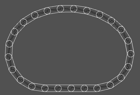
A blob made of individual particles

As constraints are processed sequentially, resolving a latter constraint may put a former one into an offending state again. Therefore, the constraint solver is executed in a loop, where the numIterations parameter can be tweaked. Increasing this parameter allows the simulation to converge to a more correct result at the expense of performance.

Having resolved all the constraints, the final part of the algorithm updates the particles’ velocities. The velocity is the particle’s displacement during the current time step, divided by the same time step. This is the reason we kept the original position thus far. Updating a particle’s velocity this way, we are implicitly applying impulses as we are resolving any collisions or other constraints.

That wraps it up for today’s post. You may want to refer to this paper for more information on the algorithm. In the upcoming posts we will cover the constraints and collision detection.

Happy coding.

Apply for the new CLIK Dashboard for game developers

Publish your game with CrazyLabs